39 how to add two data labels in excel pie chart

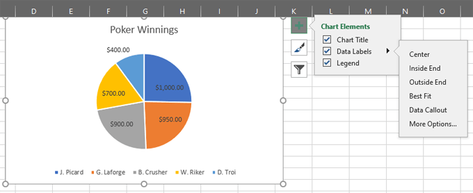
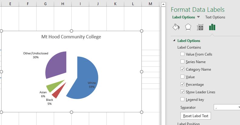
How to Make a Pie Chart with Multiple Data in Excel (2 Ways) - ExcelDemy First, to add Data Labels, click on the Plus sign as marked in the following picture. After that, check the box of Data Labels. At this stage, you will be able to see that all of your data has labels now. Next, right-click on any of the labels and select Format Data Labels. After that, a new dialogue box named Format Data Labels will pop up. How to Add Gridlines in a Chart in Excel? 2 Easy Ways! Of course, you have the option to add data labels as well, but in many cases, having too many data labels can make the chart look cluttered. So having gridlines can be useful in such cases. Let us now see two ways to insert major and minor gridlines in Excel. Method 1: Using the Chart Elements Button to Add and Format Gridlines

How to Add Data Labels to an Excel 2010 Chart - dummies On the Chart Tools Layout tab, click Data Labels→More Data Label Options. The Format Data Labels dialog box appears. You can use the options on the Label Options, Number, Fill, Border Color, Border Styles, Shadow, Glow and Soft Edges, 3-D Format, and Alignment tabs to customize the appearance and position of the data labels.

How to add two data labels in excel pie chart

How to Customize Your Excel Pivot Chart Data Labels - dummies To add data labels, just select the command that corresponds to the location you want. To remove the labels, select the None command. If you want to specify what Excel should use for the data label, choose the More Data Labels Options command from the Data Labels menu. Excel displays the Format Data Labels pane. How to Show Percentage in Excel Pie Chart (3 Ways) Jul 03, 2022 · Another way of showing percentages in a pie chart is to use the Format Data Labels option. We can open the Format Data Labels window in the following two ways. 2.1 Using Chart Elements. To active the Format Data Labels window, follow the simple steps below. Steps: Click on the pie chart to make it active. Add Data Points to Existing Chart – Excel & Google Sheets Similar to Excel, create a line graph based on the first two columns (Months & Items Sold) Right click on graph; Select Data Range . 3. Select Add Series. 4. Click box for Select a Data Range. 5. Highlight new column and click OK. Final Graph with Single Data Point

How to add two data labels in excel pie chart. Pie Chart Examples | Types of Pie Charts in Excel with Examples Now our task is to add the Data series to the PIE chart divisions. Click on the PIE chart so that the chart will get a highlight, as shown below. Right-click and choose the “Add Data Labels “option for additional drop-down options. How to Make a Pie Chart in Excel (Only Guide You Need) Jul 13, 2022 · Read More: How to Make Pie Chart in Excel with Subcategories (2 Quick Methods) Conclusion. Hope after reading this article you will not face any difficulties with the pie chart. This article covers all the necessary things regarding Excel Pie Chart. Stay tuned for more useful articles. Let us know what problems do you face with Excel Pie Chart. How To Show Two Sets of Data on One Graph in Excel Below are steps you can use to help add two sets of data to a graph in Excel: 1. Enter data in the Excel spreadsheet you want on the graph. To create a graph with data on it in Excel, the data has to be represented in the spreadsheet. For multiple variables that you want to see plotted on the same graph, entering the values into different ... excel - Positioning data labels in pie chart - Stack Overflow Positioning data labels in pie chart. I'm trying to format some charts I have, using VBA. To get started I recorded a macro of me doing what I wanted, to have an idea of what methods I'd want etc. The recorded macro looks like this - I'm including the whole thing, though the line to pay attention to is Selection.Position = xlLabelPositionCenter.

Create two data labels in pie chart? | MrExcel Message Board You have already figured out how to add an image that fills the sector of the pie chart but as far as I know you cannot add an icon or image over the actual pie chart sector, in such a way that it adjusts with the values. If you add it as a static image next to the legend, at least the legend does not move when the values change. Cheers. How to add or move data labels in Excel chart? - ExtendOffice In Excel 2013 or 2016. 1. Click the chart to show the Chart Elements button . 2. Then click the Chart Elements, and check Data Labels, then you can click the arrow to choose an option about the data labels in the sub menu. See screenshot: In Excel 2010 or 2007. 1. click on the chart to show the Layout tab in the Chart Tools group. See screenshot: 2. Then click Data Labels, and select one type of data labels as you need. See screenshot: Improve your X Y Scatter Chart with custom data labels - Get … 06-05-2021 · Thank you for your Excel 2010 workaround for custom data labels in XY scatter charts. It basically works for me until I insert a new row in the worksheet associated with the chart. Doing so breaks the absolute references to data labels after the inserted row and Excel won't let me change the data labels to relative references. How to Create and Format a Pie Chart in Excel - Lifewire To add data labels to a pie chart: Select the plot area of the pie chart. Right-click the chart. Select Add Data Labels . Select Add Data Labels. In this example, the sales for each cookie is added to the slices of the pie chart. Change Colors

Add data labels and callouts to charts in Excel 365 - EasyTweaks.com Step #1: After generating the chart in Excel, right-click anywhere within the chart and select Add labels . Note that you can also select the very handy option of Adding data Callouts. Possible to add second data label to pie chart? - excelforum.com Re: Possible to add second data label to pie chart? Create the composite label in a worksheet column by concatenating the data in other cells and the nextline character, CHR (10). Now, use this composite label column as the source for Rob Bovey's add-in. -- Regards, Tushar Mehta Excel, PowerPoint, and VBA add-ins, tutorials How to Make a Pie Chart in Excel (Only Guide You Need) 13-07-2022 · You can add an additional pie/bar chart with your pie chart in Excel. This option is useful when you have too much data in your analysis and you want some of your data to be categorized under a single data. There are two subcategories of Excel Pie chart. These subcategories are explained below. # Excel Pie of Pie Chart Add Data Points to Existing Chart – Excel & Google Sheets Show Percentage in Pie Chart: Dot Plot: Q-Q Plot: Log-Log Plot: Normal Probability Plot: ... Export Chart as PDF: Add Axis Labels: Add Secondary Axis: Change Chart Series Name: ... This tutorial will demonstrate how to add a Single Data Point to Graph in Excel & Google Sheets. Add a Single Data Point in Graph in Excel Creating your Graph.

How to Make a Pie Chart in Excel & Add Rich Data Labels to The Chart!

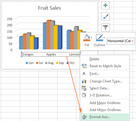
Excel charts: add title, customize chart axis, legend and data labels Click anywhere within your Excel chart, then click the Chart Elements button and check the Axis Titles box. If you want to display the title only for one axis, either horizontal or vertical, click the arrow next to Axis Titles and clear one of the boxes: Click the axis title box on the chart, and type the text.

How to Make a Pie Chart in Excel

Adding data labels to a pie chart - Excel General - OzGrid Free Excel ... With ActiveChart.SeriesCollection(1) ' HasDataLabels is a valid property .HasDataLabels = True ' XL2000 pie chart .ApplyDataLabels Type:=xlDataLabelsShowPercent _ , AutoText:=True, LegendKey:=False, HasLeaderLines:=True ' XL2003 pie chart ' .ApplyDataLabels AutoText:=True, LegendKey:= _ ' False, HasLeaderLines:=True, ShowSeriesName:=True, 'ShowCategoryName:=True _ ' , ShowValue:=True, ShowPercentage:=True, 'ShowBubbleSize:=False, _ ' Separator:=", " With .DataLabels .Font.Bold = True With ...

How to Make a Pie Chart in Excel

How to make a pie chart with two sets of data in Excel - Quora Answer: A pie chart isn't meant to show two sets of data. The pie is 100% of the data and the slices are portions representing what part of the whole each category represents. What are you trying to convey with two datasets? Is it possible you want to make two pie charts side-by-side so people ca...

How to Make a Pie Chart in Excel & Add Rich Data Labels to The Chart!

Pie Chart Examples | Types of Pie Charts in Excel with Examples Now our task is to add the Data series to the PIE chart divisions. ... pie chart, we will have two pie charts. The first one is a normal Pie chart, and the second one is a subset of the main pie chart. If we add the labels, ... Here we discuss Types of Pie Chart in Excel along with practical examples and downloadable excel template.

How to insert data labels to a Pie chart in Excel 2013 - YouTube

How to add two data labels for the same data on a pie chart? : excel Consider using two sheets, a "Calculation" sheet and your "Dashboard" sheet. Create your pie graph as usual on the "Dashboard" sheet, but remove all labels. Adjust the colors as desired. On your "Calculation sheet, create the text for your percentage label and your ratio label. For example, the first pie chart charts the data 46 and 76.

34 How To Label A Chart In Excel - Label Ideas 2020

Pie Chart in Excel | How to Create Pie Chart - EDUCBA Step 1: Select the data to go to Insert, click on PIE, and select 3-D pie chart. Step 2: Now, it instantly creates the 3-D pie chart for you. Step 3: Right-click on the pie and select Add Data Labels. This will add all the values we are showing on the slices of the pie.

Microsoft Excel Tutorials: Add Data Labels to a Pie Chart

How to add data labels from different column in an Excel chart? 1. Right click the data series in the chart, and select Add Data Labels > Add Data Labels from the context menu to add data labels. 2. Click any data label to select all data labels, and then click the specified data label to select it only in the chart. 3.

Excel charts: add title, customize chart axis, legend and data labels

How to Create Bar of Pie Chart in Excel? Step-by-Step Excel lets us add our own customizations to the Bar of Pie chart. For example, it lets us specify how we want the portions to get split between the pie and the stacked bar. It also lets us specify whether we want to display data labels, what data labels we want to be displayed as well as what formatting and styling we want to apply to the labels.

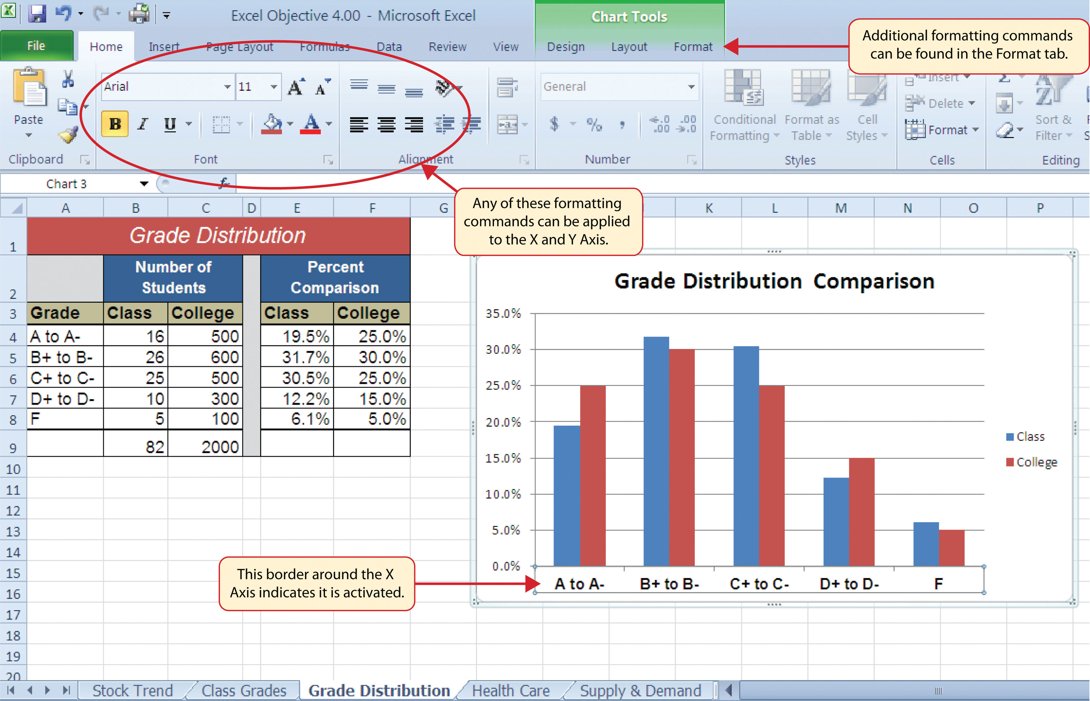
4.1 Choosing a Chart Type – Beginning Excel, First Edition

How to add live total labels to graphs and charts in Excel and ... Step 2: Update your chart type. Exit the data editor, or click away from your table in Excel, and right click on your chart again. Select Change Chart Type and select Combo from the very bottom of the list. Change the "Total" series from a Stacked Column to a Line chart. Press OK.

Advanced Graphs Using Excel : Creating fancy looking pie charts in excel 2013

How To Make a Pie Chart in Excel (With Tips) | Indeed.com Select the information and create the chart. Using your mouse, click on the cell in the top left corner and drag until you've highlighted each cell with a category or number in it. Next, click "Insert" at the top left of your window. Depending on the version, you might select "Insert pie or doughnut chart" or an icon of a pie chart, which opens ...

32 How To Add Y Axis Label In Excel - Labels Database 2020

Create a pie chart from distinct values in one column by grouping data … Select your data (both columns) and create a Pivot Table: On the Insert tab click on the PivotTable | Pivot Table (you can create it on the same worksheet or on a new sheet) On the PivotTable Field List drag Country to Row Labels and Count to Values if Excel doesn't automatically. Now select the pivot table data and create your pie chart as ...

How to Make a Pie Chart in Excel & Add Rich Data Labels to The Chart!

Add a DATA LABEL to ONE POINT on a chart in Excel All the data points will be highlighted. Click again on the single point that you want to add a data label to. Right-click and select ' Add data label '. This is the key step! Right-click again on the data point itself (not the label) and select ' Format data label '. You can now configure the label as required — select the content of ...

How to Make a Pie Chart in Excel & Add Rich Data Labels to The Chart!

Pie of Pie Chart in Excel - Inserting, Customizing - Excel Unlocked Inserting a Pie of Pie Chart. Let us say we have the sales of different items of a bakery. Below is the data:-. To insert a Pie of Pie chart:-. Select the data range A1:B7. Enter in the Insert Tab. Select the Pie button, in the charts group. Select Pie of Pie chart in the 2D chart section.

Excel Chart Data Series, Data Points, and Data Labels

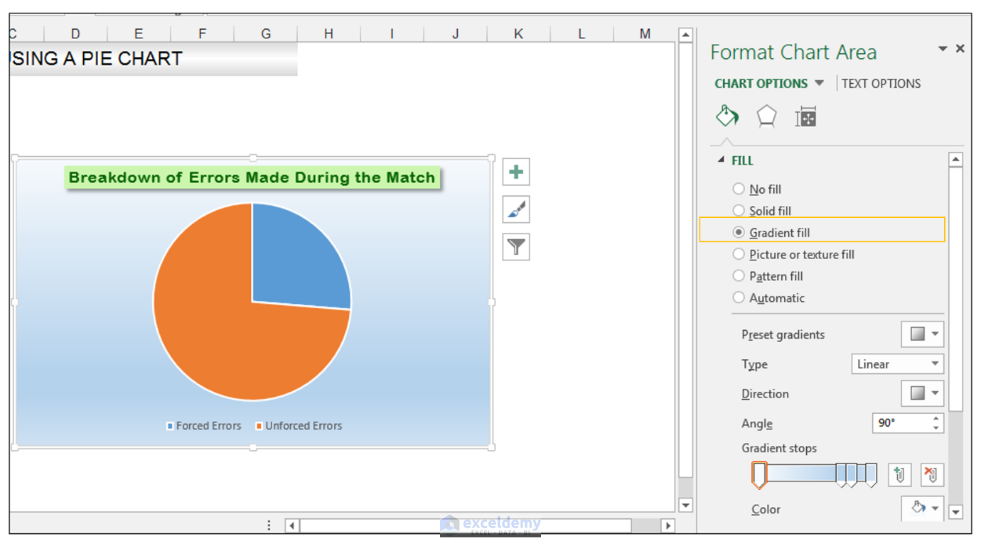
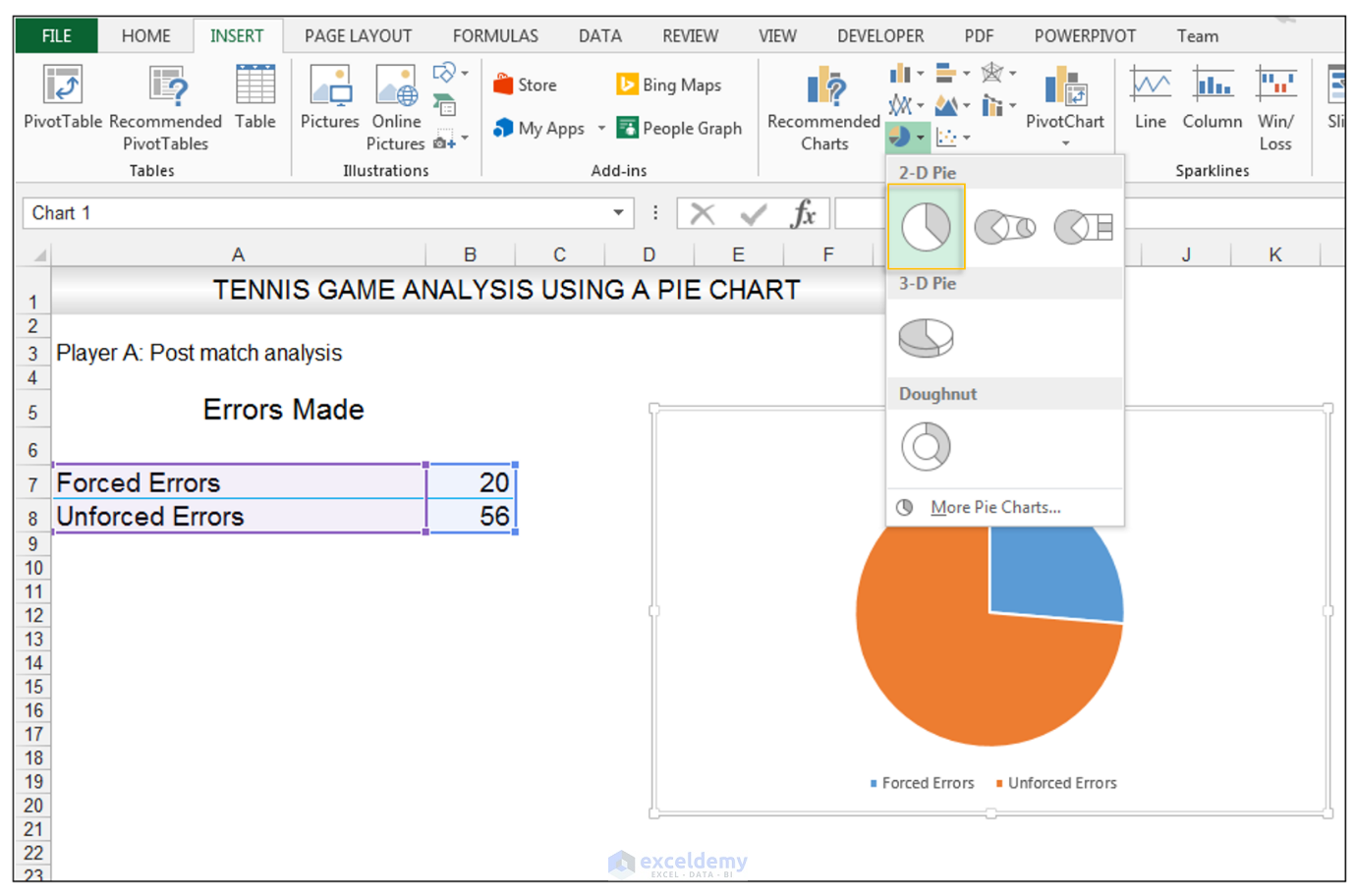
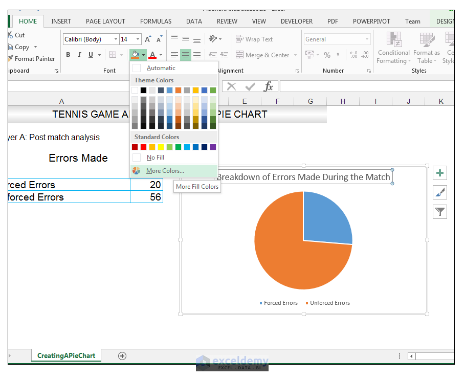
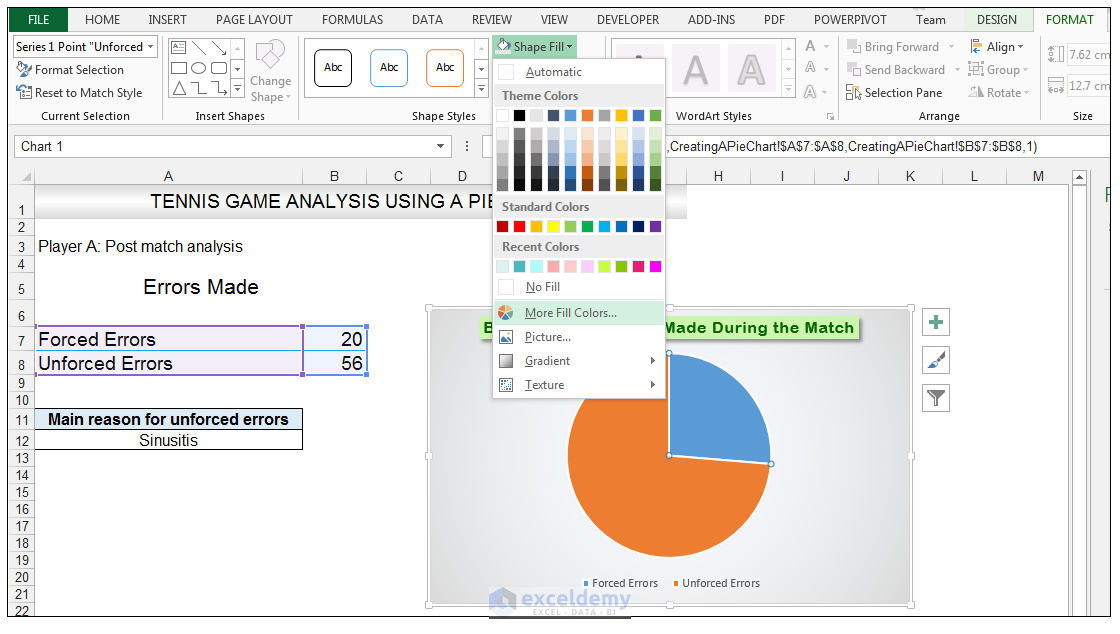
How to Make a Pie Chart in Excel & Add Rich Data Labels to The Chart! 1) Select the data. 2) Go to Insert> Charts> click on the drop-down arrow next to Pie Chart and under 2-D Pie, select the Pie Chart, shown below. 3) Chang the chart title to Breakdown of Errors Made During the Match, by clicking on it and typing the new title.

How to Make a Pie Chart in Excel & Add Rich Data Labels to The Chart!

Edit titles or data labels in a chart - support.microsoft.com The first click selects the data labels for the whole data series, and the second click selects the individual data label. Click again to place the title or data label in editing mode, drag to select the text that you want to change, type the new text or value.

Share :